• online
• 1.0

L-systems in J

R.E. Boss (r.e.boss@planet.nl)

Introduction

There are not many examples of repeated squaring [1], but I stumbled upon a new one in 2006, solving a problem posed by Bron [2]. To explain it I use some examples and some theory, but then a new method is introduced in J. The term L-system in the title is short for Lindenmayer system [3] [4].

Rabbit sequence

This is an infinite sequence [5] of booleans which has the property that if one changes each 0 to a 1 and every 1 to the pair 1 0 , the sequence does not change.

1 0 1 1 0 1 0 1 1 0 1 1 0 1 0 1 1 0 1 0 1 1 0 1 1 0 1 0 1 1 0 1 1 0 1 0 1
1 0 1 0 1 1 0 1 1 0 1 ….

Notice that this is the Algae example [6] in [3].

Lindenmayer systems

An L-system is a parallel rewriting system, i.e. consisting of an alphabet V of symbols which can be replaced, a set of (production) rules P such that each rule replaces a particular symbol of V in a string of symbols (from V), and an initial symbol S to which the rules subsequently are applied.

All rules are applied at the same time, therefore the system is parallel.

In fact P is a mapping from V → V*, the set of all strings with symbols from V, including the empty string. If for some a ∈ V one has P(a)=s, with s some string, this is also denoted by a → s.

If for a symbol c in V one has P(c) = c, then c is called a constant.

If a symbol in V is not a constant, then it is called a variable.

In the example of the rabbit sequence, V is the set of booleans {0,1}.

The rules are P(0) = 1 and P(1)= 1 0 and the initial symbol S is 0.

L-systems in J

To apply J [7] in producing an L-system, I prefer the alphabet V to be a set of integers, say {0,1,…,n-1}, such that(mostly) S is represented by 0.

Then the mapping P can be represented by an array of boxes, all of which contain an array of integers form V. The production rules are then P(k) = ;k{P.

So for the rabbit sequence we get V =: 0 1, S =: 0 and P =: 1; 1 0 .

Now the verb to produce the next generations of S is easy to construct:

    P {~ S
+-+
|1|
+-+

   P {~^:2 S
+---+
|1 0|
+---+

But after that we get a problem:

   P {~^:3 S
|length error
|   P    {~^:3 S

This can easily be repaired by the following verb:

   P ([:; {~)^:3 S
1 0 1

And now we can get a rabbit sequence of any length:

   P ([:; {~)^:20 S
1 0 1 1 0 1 0 1 1 0 1 1 0 1 0 1 1 0 1 0 1 1 0 1 1 0 1 0 1 1 0 1 1 0 1 0 1
1 0 1 0 1 1 0 1 1 0 1 0 1 1 0 1 0 1 1 0 1 1 0 1 0 1 1 0 1 1 0 1 0 1 1 0 1
0 1 1 0 1 1 0 1 0 1 1 0 1 1 0 1 0 1 1 0 1 0 1 1 0 1 1 0 1 0 1 1 0 1 0 1 1
0 1 1 0 1 0 1 1 0 1 1 0 1 0 1 1 0 …

Which can be given a bit more sophisticated by P ([:; {~)^:(]`(S"_)) 20

Notice that if the production rules all have the same length, no boxing is needed, in which case the ; in the expression is replaced by a , .

More examples

Some examples from [3] are Cantor dust [7] and Koch curve [8].

The first is given in J by V =: 0 1, S =: 0 and P=: 0 1 0; 1 1 1 so

   P ([:; {~)^:(]`(S"_)) 3
0 1 0 1 1 1 0 1 0 1 1 1 1 1 1 1 1 1 0 1 0 1 1 1 0 1 0

Where 0 represents black and 1 represents white.

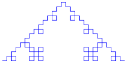
The Koch curve [8] is given by

   V=:0 1 2,  S =: 0

and

   P=: 0 1 0 2 0 2 0 1 0; 1; 2

   P ([:; {~)^:(]`(S"_)) 3
0 1 0 2 0 2 0 1 0 1 0 1 0 2 0 2 0 1 0 2 0 1 0 2 0 2 0 1 0 2 0 1 0 2 0 2 0
1 0 1 0 1 0 2 0 2 0 1 0 1 0 1 0 2 0 2 0 1 0 1 0 1 0 2 0 2 0 1 0 2 0 1 0 2
0 2 0 1 0 2 0 1 0 2 0 2 0 1 0 1 0 1 0 2 0 2 0 1 0 2 0 1 0 2 0 2 0 1 0 1 0
1 0 2 0 2 0 1 0 2 0 1 0 2 0 2 0 1 …

With the graph below.

Given these examples, anybody can make her own.

Repeated squaring

Now the question (with which I perhaps whetted your appetite) in the introduction is still open, what about repeated squaring?

If you look at the verb P ([:; {~)^:(]`(S"_)) it is obvious the behaviour is rather linear. In each iteration a string is used to apply P on the individual symbols of the string and the results are concatenated.

Now consider P^k which is the mapping applied k times (on S which is 0). It is easy to construct in J by (;@:{&.> <)^:(k-1)~ P .

If we apply this to the rabbit sequence (V =: 0 1, S =: 0,P =: 1; 1 0 ) we get

   (;@:{&.> <)^:(<4)~ P
+---------+---------------+
|1        |1 0            |
+---------+---------------+
|1 0      |1 0 1          |
+---------+---------------+
|1 0 1    |1 0 1 1 0      |
+---------+---------------+
|1 0 1 1 0|1 0 1 1 0 1 0 1|
+---------+---------------+

As soon as (some of) these P^k are known, repeated squaring can start:

binind=: I.@|.@#: NB. The binary indices are determined

appl=: (;@:{&.> <) NB. Applying the main verb

rs=: 4 : '> {. appl/ appl^:(binind y) x' NB. x equals P and y is the generation giving the complete solution

The figures show that the performance is what you would expect, much better, while the output is the same:

   ts'P ([:; {~)^:(]`(S"_))35'
0.50670696 1.6777933e8

   ts'P rs 35'
0.022058907 79695232

   (rs-:P ([:; {~)^:(]`(S"_))]) 35
1

In this example we can do even better, since for the rabbit sequence we have P^k+1 = P^k , P^k-1 , indeed Fibonacci!

   ts'3 : '';|. appl/ appl^:(]`(P"_)) binind y-2''35'
0.012114756 46154880

So this gives a solution which is about 40 times as fast and 3.5 times as lean as the original one.

Final example, Gray codes

The last I owe the reader was the solution I found for the problem of Bron [2]. He asked for the most efficient verb to generate the Gray code, see [9] and [10]. Fortunately he also allowed to generate the decimal values of that code, which for the first 64 numbers look like:

G=: 0 1 3 2 6 7 5 4 12 13 15 14 10 11 9 8 24 25 27 26 30 31 29 28 20 21 23
22 18 19 17 16 48 49 51 50 54 55 53 52 60 61 63 62 58 59 57 56 40 41 43 42
46 47 45 44 36 37 39 38 34 35 33 32 .

The fractal structure of the code becomes apparent if you do

   2-~/\ G
1 2 _1 4 1 _2 _1 8 1 2 _1 _4 1 _2 _1 16 1 2 _1 4 1 _2 _1 _8 1 2 _1 _4 1 _2
_1 32 1 2 _1 4 1 _2 _1 8 1 2 _1 _4 1 _2 _1 _16 1 2 _1 4 1 _2 _1 _8 1 2 _1
_4 1 _2 _1 .

To not let grow the numbers too quickly, I transformed it in

   G1=: (** 2^. 2* |) 2-~/\ 64{.G
1 2 _1 3 1 _2 _1 4 1 2 _1 _3 1 _2 _1 5 1 2 _1 3 1 _2 _1 _4 1 2 _1 _3 1 _2
_1 6 1 2 _1 3 1 _2 _1 4 1 2 _1 _3 1 _2 _1 _5 1 2 _1 3 1 _2 _1 _4 1 2 _1
_3 1 _2 _1 .

By the way, this representation of the (binary reflected) Gray code has a very useful interpretation: each number gives by its absolute value the coordinate where two consecutive code words differ, and by its sign how they differ: + if 0→1 and – if 1→0.

So I defined V to be the set of integers and S=:1 . But most important was P. To produce G1, I defined

   P=: 1; 1 2 _1; 3; 4; 5; 6;(…); _6; _5; _4; _3;1 _2 _1

Notice that in fact P is infinite, which is indicated by the (…).

Notice also that (P{~ –n) -: |.- n{ P for n > 0, so in general we have P=:3 :'1; (, [:|. -@|.&.>) 1 2 _1; ;/3+ i.y'n for some n, like

   [P=:3 :'1; (, [:|. -@|.&.>) 1 2 _1; ;/3+ i.y'6
+-+------+-+-+-+-+-+-+--+--+--+--+--+--+-------+
|1|1 2 _1|3|4|5|6|7|8|_8|_7|_6|_5|_4|_3|1 _2 _1|
+-+------+-+-+-+-+-+-+--+--+--+--+--+--+-------+

The only thing one has to do is to transform this resulting fractal in the Gray code again, ie to invert (** 2^. 2* |) and precede it by 0 :

   +/\0,(** 2%~ 2^|) P rs 6
0 1 3 2 6 7 5 4 12 13 15 14 10 11 9 8 24 25 27 26 30 31 29 28 20 21 23 22
18 19 17 16 48 49 51 50 54 55 53 52 60 61 63 62 58 59 57 56 40 41 43 42
46 47 45 44 36 37 39 38 34 35 33 32

which is equal to the original G. This, in principle, gives the impressive performance results in [2].

Conclusions

Using L-systems in J is a powerful technique for generating all kinds of fractal like structures. In a next paper I will describe how to transform these arrays in nice graphs using the plot facility of J.

Bibliography

1. RepeatedSquaring.
   [Online]. http://www.jsoftware.com/jwiki/Essays/Repeated%20Squaring.
2. Bron. [Online]. http://www.jsoftware.com/jwiki/Puzzles/Gray%20Code.
3. Lindenmayer1. [Online]. http://en.wikipedia.org/wiki/L-system.
4. Lindenmayer2. [Online]. http://mathworld.wolfram.com/LindenmayerSystem.html.
5. RabbitSequence.
   [Online]. http://www.maths.surrey.ac.uk/hosted-sites/R.Knott/Fibonacci/fibrab.html.
6. Algae. [Online]. http://en.wikipedia.org/wiki/L-system#Example_1:_Algae.
7. CantorDust. [Online]. http://en.wikipedia.org/wiki/L-system#Example_3:_Cantor_dust.
8. KochCurve. [Online]. http://en.wikipedia.org/wiki/L-system#Example_4:_Koch_curve.
9. GrayCode1. [Online]. http://en.wikipedia.org/wiki/Gray_code.
10. GrayCode2. [Online]. http://www.jsoftware.com/jwiki/Essays/Gray%20Code.